Category Archives: Uncategorized

In Simulating Minds Alvin Goldman develops his account of “mindreading”, i.e. the conditions under which we humans attribute to one another beliefs and desires (and feelings, high-level decisions, actions, perceivings, and so on). This isn’t an epistemological theory, of how our beliefs about other minds are justified, but an empirical theory of how we in fact go about the task. Accordingly, evidence from neuroscience, cognitive science and psychology looms large.

Goldman sees himself as defending a “simulation theory”, according to which the central mechanism for mindreading others is one where we use our own processes for forming beliefs and desires (on the basis of evidential inputs) or forming decisions (on the basis of beliefs of desires). The idea is that we have the capacity to deploy these processes “offline”, inputting pretend-evidence into our usual belief-and-desire forming processes, and extracting pretend-belief and pretend-desire. Or, indeed, inputting pretend-belief and pretend-desire into our normal decision-making procedures and extracting pretend-decisions. According to Goodman, a paradigmatic belief attribution might first, identify the presumed evidence of our target; second, use the simulation routine to generate pretend-belief that p, third, use an introspection/classification/attribution routine, with the overall upshot of that we form the belief that our target believes that p.

Goldman thinks of this only as a description of our “fundamental and default” mode of mindreading. Presumably the beliefs that are generated by the three-step procedure will, in the usual course of events, be brought into contact with other beliefs that we might have about the target. For example, we might have been told by a reliable source that the target definitely did not believe that p, or we might have general inductive evidence that people don’t believe that p. We might acquire information that the target is a spy who’s aiming to fool us into believing that p. Acknowledging that we are sensitive to these kind of rebutting or undercutting defeaters are quite consistent with Goldman’s theory. The point, I take it, of his describing the simulation mechanism as “default” is to allow its outputs to be weighed against all sorts of other evidence which might lead to us not ending up with the beliefs that simulation procedures direct us to. Goldman can also acknowledge that we sometimes form beliefs about others’ mental states through testimony or induction, without any role for simulation. The point, I take it, of his describing simulation-based mind-reading as “fundamental” is to acknowledge that we form beliefs about others mental states by induction and testimony, but to categorize these as subordinate to the mindreading method he is describing. All this seems pretty commonsensical–a basic but compelling foundationalist thought is that if we trace back the chains of testimony and induction, on pain of regress, we need some non-inductive or non-testimonial way of forming beliefs about others’ beliefs. Mindreading Goldman-style is a natural candidate.

A pure form of simulationism would claim that it can produce attributions of belief and desire to a target quite independently any prior views the attributer has about the target’s beliefs and desires. Pure simulationism is quite compatible with the kind of story just told about the need to integrate the outputs of simulation with prior views about the target’s psychology, but it would see that as strictly optional. But Goldman doesn’t endorse pure simulationism. Indeed, there are a couple of places where he implies that prior beliefs about the target’s psychology (either specific or in the form of generics that cover all targets) are required in order to implement simulation. The central example of this involves mindreading by retrodiction. Suppose the information we have about a target includes how they behave. We want to let this inform our opinion about what their beliefs and desires are. The interpreter has at their disposal their decision-making process, which takes in beliefs and desires and choice situations and spits out decisions. But that mechanism runs in the wrong direction, for the present interpretive problem–one can’t directly feed in pretended-decisions and get out pretended-beliefs and desires. Goldman conjectures that the simulationist instead proceed by a process of “generate and test”. We start from a hypothesis about what the target believes/desires, convert that into pretend-believes and desires which are fed, offline, into our own decision making procedure, resulting in pretend-decisions. If this matches the observed decisions, the hypothesis has passed the test and can be classified and attributed to the target. If not, we need to loop back to generate a new hypothesis. This generate-and-test loop for retrodictive mindreading involves simulation, but the “generation” (and regeneration upon failure) is not explained by simulative means. Some other explanation is owing about how we generate the hypothesis. And Goldman suggests that here we will appeal to our prior beliefs about what the target’s psychology is likely to be. If prior beliefs about target psychology are essential to retrodictive mindreading, as this suggests, then Goldman’s account is not pure simulationism. Goldman acknowledges and embraces this—he thinks that what we will end up is a compound story that involves elements of theorizing as well as simulating within the “fundamental and default” story about how we attribute higher mental states to others. (This concession generates some dialetical vulnerabilities for Goldman’s wider project, as Carruthers points out in his NDPR review of Goldman’s book.)

As I see it, the significant issue here is not that we *sometimes* use prior knowledge about others to generate hypotheses about their mental states which are fed into the generate-and-test simulation routine. That’s as unproblematic as the idea that the outputs of simulation routines need to be integrated into prior opinions about others, before they are ultimately endorsed. What’s significant is that it is looking like such prior knowledge is, for all Goldman says, always required for simulationist mindreading, to generate the hypotheses for retrodictive testing. And that means that some other method of arriving at beliefs about others’ psychology needs to be co-fundamental with the simulationist method, on pain of regress.

I want to describe a purer simulationism. Crucial to this is to think about the way the predictive and retrodictive mindreading combine. In essence, the idea will be that predictive mindreading can generate the hypotheses that are tested by retrodiction. Let’s see how that might work.

Rather than assume we *either* have information about a target’s evidential situation, or about their behaviour, let’s suppose (more realistically) that we have some information about both. Given this, here’s a doubly simulationist proposal. First, identify the target’s evidence, and run a simulation with those as pretend-outputs, to arrive at an initial set of “pretend-beliefs and desires”. This generates an initial “anchor” hypothesis about what the target’s psychology is like. But we haven’t yet brought to bear what is known about their behaviour. So we test the anchor hypothesis by feeding it into our decision-making process, arriving at pretend-decisions/behaviour. In the good case, the pretend-decisions and their behavioural signature match the behaviour that is observed, and we’ve just run a complete double cycle of simulationist mindreading, and are ready to classify and attribute the attitudes to the target.

In the bad case, though, there’s a mismatch between reality and the simulated decisions generated by the anchor hypothesis. In this case, we need to revise the hypothesis and try again. The pure simulationist at this point can conjecture that there is a fixed search space—an list of modifications to try, in order to generate a revised hypothesis. Picturesequely, we can imagine a space of possible interpretations, ordered by similarity to one another. The anchor interpretation generated by simulating the target’s reaction to evidence gives a starting point to be fed into the simulation-test-procedure to see if the decisions it predicts match those observed. If that fails to pass the test, then we move to try a sphere of closest interpretations to the anchor, and try those. If that fails, we move yet further out, and so on—until we run out of patience and give up. This is a hypothesis generating procedure that does not presuppose any prior information about the target’s psychology or the psychologies of agents in general, but only a measure of similarity between interpretations that defines a search method.

What would be the upshot of this combined way of mindreading? When starting with information about both evidential input and behavioural output of a target, we’d end up attributing that belief/desire psychology which is most similar (among psychologies that, under simulation, match the observed behaviour) to the belief/desire psychology produced by simulation of the evidence.

Just as before, this candidate psychological attribution will be tempered (rebutted/undercut/modified) by anything we happen to know about the target, and various stages in the pure form of the mindreading method can substituted by opinions we happen to hold. But even granted all this, what we have, I claim, is a possible pure simulationist routine for mindreading, one that could in principle be run entirely independently of prior views about what beliefs and desires the target has. It could, indeed, be the way we form the initial beliefs that are grist to the mill of induction and IBE by which we form psychological generalizations of that kind, within a foundationalist epistemology.

This last claim requires that prior opinion about beliefs/desires of others isn’t presupposed anywhere else in the method. Carruthers in his review of Goldman suggests that there’s another place where prior opinion matters—even predictive simulation requires we identify what the target’s evidence is, in order that this converted to pretend-evidence to be fed into our belief-forming mechanisms. That worry doesn’t seem so serious to me. As ever, the pure simulationist can concede it’s possible for prior beliefs to determine what we should take the pretend-evidence to be, to feed into the simulationist mindreading. But Goldman also defends “lower level”, automatic processes of mindreading, whereby visual information the attributer has about a target involuntarily triggers a “mirroring” within the attributer of the target’s perceptual processes. So this seems like a route entirely independent of beliefs about evidence, by which an Goldman style simulationist interpreter can identify the evidential situation of a subject, and then, by secondary “higher level” simulation, generate beliefs about what propositional attitudes they possess. The same goes for the identification of behaviour.

A second place where prior opinion might matter is the following. Goldman appeals to a distinction between those beliefs/desires of the attributer that are ‘quarantined’ (not used as auxiliary premises in simulating belief-formation/decisions) and those beliefs/desires that are not quarantined. What that distinction is, or should be, and whether *that* depends on prior opinion about targets, is I think a central question for the Goldman-style simulationist. And it’s another possible loci for simulation being infected by opinion. If the idea is that we quarantine those attitudes of ours we know to be idiosyncratic, then knowledge of how our psychological compares to those of others would be central to the operation of simulation itself. I think this, too, can be resisted, and a different story about quarantine given, but that is a matter for another time.

There are two things I take away from this discussion. The first is that it’s at least open to Goldman to develop a pure form of simulationism on which simulation is the *only* fundamental/default mindreading process, albeit one that only be operates in a “pure” way in the idealized limit. The second thing I take away from the discussion is the recipe that simulationism predicts, in that idealized limit. That is: in the ideal limit we attribute the behaviour-simulating interpretation which is most similar to the anchor interpretation simulated by the target’s evidence. That last bit of information is the sort of thing that is crucial to *my* larger project right now.

In the last post, I described an epistemic bargaining problem, and applied Nash’s solution to it. That gave me a characterization of a compromise “team credence”, as that credence which maximizes a certain function of the team members’ epistemic utilities. This post now describes more directly what that team credence will be (for now, I only consider the special case where the team credence concerns a single proposition). Here’s the TL;DR: so long as two agents are each sufficiently epistemically motivated to find a compromise, then they will compromise on a team credence that is the linear average of their individual credences iff they are equally motivated to find a compromise. If there is an imbalance of motivation, the compromise will be strictly between the linear average and the starting credence of the agent who is less motivated by finding the team credence.

To recap, we had a set of team members. These team members each assign “expected epistemic utility” to possible credal states (including credal states that concern only attitudes to the single proposition p). Expected epistemic utility is assumed to be the expected accuracy of the target credal state x, and inaccuracy is assumed to be measured by the Brier score if p is true, if p is false (to get a measure of accuracy, subtract inaccuracy from 1). For an agent whose own credal state is a, it’s a familiar piece of bookwork to show this implies that the epistemic utility of a credal state x(p) is —one minus the square euclidean distance between the agent’s own a(p) and the target credence x(p). From now on, I’ll drop the indexing to p, since only one proposition will be at issue throughout.

The epistemic decision facing the several agents is this: they can form a team credence in p with a specific value, so long as all cooperate. But if any one dissents, no team credence is formed. The situation where no team credence is formed is assumed to have a certain epistemic utility for the epistemic utility for agent A (who has credal state a). So forming the specific team credence x will be worthwhile from A’s perspective if and only if the epistemic utility (expected accuracy) of forming that team credence is greater than the default, i.e. iff . Now, we may be able to find a possible credal state $d_a$ which the agent ranks equally with the default credal state, . You can think of as A’s breaking point—the credence at which it’s no longer in her epistemic interests to form a team credence, since she’s indifferent between that and the default where no team credence is formed. A little rearrangement gets us to: . So really we have both an upper and lower breaking point, and within these bounds, a zone of acceptable compromises, within which a team credence will look good from that agent’s perspective.

Possible credences will be, as is standard, within the interval . may well be outside that interval. Consider, for example, the case where an agent has credence 1 or 0 in p to start with, or a situation where not forming a team credence is a true epistemic disaster, of disutility >1. It’ll be formally convenient to still talking of breaking point credences in these cases, but that’ll just be a manner of speaking.

A precondition of having a bargaining problem is that there are some potential team credences x that all team members prefer to have team credence x than the scenario where no team credence is formed. That is, for all y in the group, . That amounts to insisting that the set of open intervals have a non-empty intersection, or equivalently, where y runs over hte team members, .

That’s a lot of maths, but concretely you can think about it like this: it’ll be harder to strike a compromise on p the more distant the team member’s credences are from each other. If, however, each feels great urgency to finding a team credence, that will widen the zone of compromise from their perspective. So even if A starts with credence 1 in p, and B starts with credence 0 in p, then they will each view some compromises between the two of them as acceptable if A’s lower breaking point is higher than B’s upper breaking point. That relates to the utility/disutility of failure: if failure for A is worse than the epistemic cost of having credence 0.5 in p, and similarly for B, then credence 0.5 is a potential compromise for the two of them.

So these are the conditions for there to be a bargaining problem in the first place. If they are met, everyone wants a deal. The question that remains is which among this set they should pick. As described in the last post, if we endorse Nash’s four conditions we have an answer: the team credence will be the x that maximizes the following quantity: . Simplifying a touch, the latter curve becomes .

Before moving on, I do want to make one observation that will be important later: that the Nash compromise team credence is somewhere in . This is pretty intuitively obvious, but to argue for it formally: suppose that we have N agents with various starting credences, whose span is the interval . If the upper endpoint b is not within the intersection of the zones of compromise, then nothing above b is within this intersection either (since those constraints take the form of an intersection of open balls around points no greater than b). On the other hand, suppose that the b is contained within the intersection of all the agents’ zones of compromise. Then we can see that the Nash product cannot take its maximum value above b. That’s because b will be nearer all the starting credences than anything above b, and so every multiplicand (and hence the product) will be greater at the endpoint than it is at any point above it. The same goes, in reverse, for the other endpoint a.

So what does Nash’s maximization condition say about specific cases? One complicating factor is that this is a constrained maximization problem, over the set . So looking at the curve defined by Nash’s product alone doesn’t contain all the information we need to pick the constrained maximum. I’ll come back to this at the end, but for now, I’ll ignore the issue and concentrate on finding a local maximum of the Nash curve.

Let’s get going with the local maximization problem then, for the two-agent case. We want to find a turning point of the Nash curve . To see what’s going on with this quartic polynomial, consider a special simple case with a at 1 and b at 0, and both offsets at zero. That gives , which I’ve sketched for you (as with the other images that follow) using wolframalpha:

This polynomial has roots at 0 and 1—and every candidate team credence of course has to be within this zone. And so you can see immediately that the leading candidate to be the compromise credence will be the local maximum of this curve. To find the value of the maximum, we remember secondary school maths and set the derivative of the curve equal to zero.

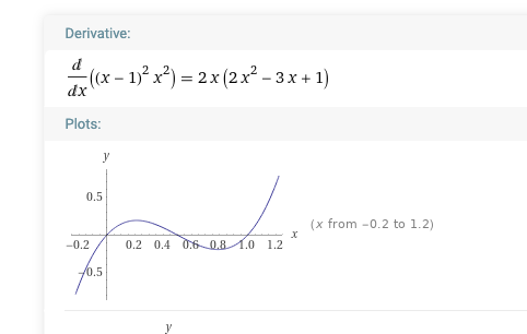
Note we can factorize the derivative as . The cubic has three roots: 0 and 1 (those are the minimum points of the original quartic curve) and 0.5.

This looks promising! Interpreting this in the epistemic bargaining way, we have started with two agents with extremal credences 1 and 0, and found that we have a local maximum for the Nash curve at their linear average. Further, this is representative of a general pattern. If you start from , then you get curves that look like distorted versions of the above, but with roots of the original curve at a and b, and a local maximum at —the linear average of the starting credences.

Things look even better when we recall that the maximum value of the Nash curve *for values of x that met the relevant constraints* was going to have to be within the interval spanned by the starting credences. For that tells us we can ignore all the curve except the bit between 0 and 1 in the extremal case (but we knew that anyway!) and between a and b in the general case. The arms of the original curve that shoot off to infinity can be ignored, therefore—and that’s one big step towards arguing that the local maximum (the turning point we’ve just calculated in this special case) is the point satisfying Nash’s conditions.

Now, this is all very well, except for the annoying fact that the simple case in question was one where , which translates to both agents having a null zone of compromise (in terms of breaking points: the breaking point credence for each agent is the point at which they’re at). There’s no non-trivial bargaining problem at all here! So that there’s a local maximum of the curve at the linear average doesn’t tell us anything of interest. Bother.

But the general case can be understood in relation to this one. Again starting from extremal credences for simplicity (A having credence 1 in p, B having credence 0 in p), the non-trivial bargaining problems will take the form . Multiplying this out we have: . Differentiating this and setting the result to zero we have . This is equivalent to finding the intersection of the cubic sketched above and the linear curve . To illustrate, here’s a sketch of what happens when both parameters are set to 1. The intersection, and so the local maximum of the original curve, is the average of the two credences, at 0.5:

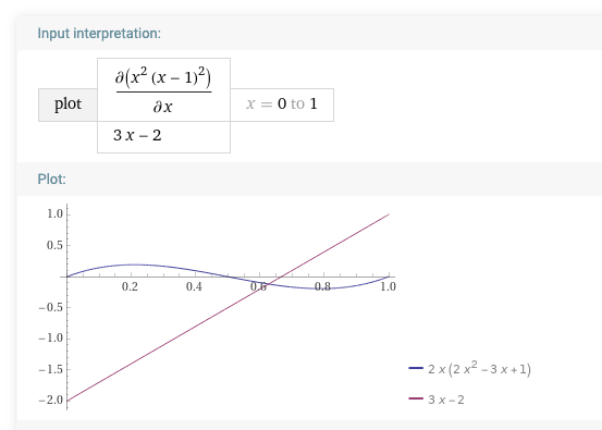
Below is the case where but . Note that the intersection is now below the linear average of the two starting credences (that makes sense: the parameters tell us that A, with full credence, is more distant from her breaking point than B, who has zero credence—or equivalently, failing to agree a team credence is in relative terms better for B than for A. So A is in the weaker bargaining position and the solution is more in line with B’s credence):

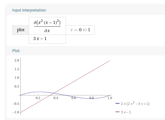
And below is what happens if we reverse the parameters, with the intersection point, as expected, nearer to the agent with less to lose, in this case, A (who had full credence):

What of the general two-agent case, where the equation for which we’re finding the local maximum is ? This time I’ll run through it algebraically. Assume without loss of generality a>b. From a note earlier, we know the compromise credence is to be found in the interval . So under what conditions is it in the top half, ? At the bottom half ? And at the midpoint ?

First, multiply out: . Second, differentiate the quartic and set the result to zero. This gives us . This is equivalent to finding the intersection of the cubic and the linear curve . The former, recall, is like a squished version of the the earlier cubic, with roots at –the middle root corresponding to the local maximum.

Now, you can eyeball the curve sketches above to convince yourself that the following biconditional: the intersection of the cubic and linear will be at an x-value within iff the linear curve intersects the x-axis within the same interval. Inverting the linear equation, we find that its intersection with the x-axis will be . That will be within the interval only if , which is to say: . Multiply out, simplify while remembering we were assuming a>b, and you will find this is equivalent to: . (Interpretation: the epistemic utility of no team credence is higher for A (at ) than for B (at )).

By similiar manipulations, we can show that the intersection of the two curves lies within only if . And the two curves intersect at iff . And given the curves intersect somewhere in the interval [b,a], and the three conditions are mutually exclusive, we can now strengthen these two conditionals to biconditionals.

To summarize: Maximizing the Nash curve over [a,b] to pick a compromise team-credence gives the linear average when the epistemic utility of failing to reach a team-credence is the same for both parties. When there is an imbalance in the epistemic utilities of failure, if we pick the team credence in the same way, we’ll get a result that is nearer the starting credence of the agent with less to lose from failure.

All this comes with the caveat mentioned earlier: I’ve been talking about how to find the maximum of the Nash curve over the whole of [a,b]. We need to also remember that we were to find the maximum over a constrained set of credences, and this might be a proper subinterval of [a,b]. At the limit, as we saw earlier, they may be no credences meeting the constraints at all. So it’s not guaranteed (yet) that the Nash compromise in all (two person, one proposition) cases satisfies the description given above. But it will meet that condition if the zones of compromise are big enough: if they are big enough that [a,b] is contained within them.

That’s enough for today! The next set of questions for this project I hope are pretty clear: Is there more to say about the case when constraints are a proper subinterval of [a,b]? How does this generalize to about the N-person case? How does this generalize to a multiple proposition case? How does it generalize to scoring rules other than the Brier score?

P.S. Thanks to Seamus Bradley and Nick Owen for discussion of this. As they noted, you can use computer assistance to find exact roots for the cubic and so the turning point of the quartic. Unfortunately, those exact roots look horrific, which pushed me towards the qualitative results reported above. I include the horror for the sake of interest, with C and D being the delta terms for a and b respectively:

P.P.S. Some further notes about the next set of questions.

(i) On the issue of when we have a well defined bargaining problem. For the two-person case, the following holds: there is a non-trivial bargaining problem when . In the special case where , that means . The compromise zone is maximal, i.e. the whole of iff .

The following graphical characterization was illuminating to me. In general, the quartic has a “W” shaped curve. For very negative values of x, then both and $(\delta_B-(x-b)^2)^2)$ are large and negative, and so their product is large and positive. For very positive values of x, both are large and again negative, so their product is large and again positive. If all roots are real, then moving from left to right, as x approaches a we get an interval where is positive and the other negative, then an interval where both are positive, and then a period when only $(\delta_B-(x-b)^2)^2)$ is positive, before both turn negative. Now note that the middle interval exactly corresponds to the values for which both agents have positive utility, and so is exactly the zone of compromise. So another characterization of the compromise zone is the area between the middle two roots of the quartic (if those roots are imaginery, there is no bargaining problem). This is important, because it illuminates why finding the local maximum is the right method–it’s because the constraints are that we only maximize in that specific interval between the middle two roots, and the maximum subject to that constraint is exactly the local maximum.

(ii) For the 3-person case, we can consider constraints and maxima. For the former, it’s a necessary condition that the most confident and least confident individual overlap, and so if we designate those a and b, we again need the following for there to be a non-trivial zone of compromise: . In addition, however, we need the zone around c to overlap this, which is a complex three case condition involving c and $latex\delta_C$. If c is at the midpoint of a and b then any nonzero will do. 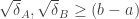Likewise, it is necessary for the compromise zone to be maximal that , and then there is a more complex condition involving c and . suffices, but e.g. if c is the midpoint then a smaller will do. Something similar happens with the general N-person case—that the zones of compromise of the extremes overlap is a necessary condition, and then there’s an array of more complex conditions for those whose credence lies between the two extremes.

The N-person case involves us finding a maximal point of a polynomial of degree 2N. The new challenge here is that there are multiple local maxima—which can all be between 0 and 1, in principle. The generalization of the point made earlier is now crucial to understand what is happening. Suppose all roots are real As we scan from left to right, we start from a point where all the multiplicands (epistemic utility difference of agents) are negative, and gradually hit points where more and more agents have positive epistemic utility difference (toggling the sign of the product, i.e. the curve, from positive to negative and back again), until eventually all multiplicands are positive. Then we continue to scan to the right more and more turn negative. The key observation is the zone of compromise for all agents are those points at which all agents have positive utility, which is the middle hump of the serpent’s back. The conditions for this existing, and for being maximal, i.e. covering , are given above. But a crucial observation is that the maximization problem is now well defined: we need to find the local maximum of this middle hump.

What are the compromise credences in these cases? Well, here’s one special case that is as you’d expect: if c is at the average of a and b, and the threatened losses are the same for a and b, then the compromise team credence will be c. If c is nearer to a than b, the credence is nearer to a than b, and vice versa. If the threatened loss is bigger for a than b, then the compromise is nearer b (if c is at the average). How these trade off, and the N-person generalization, will require more work. There’s some attractive initial hypotheses that fail. For example, in the two person case, as reported above, when the potential losses are equal, the compromise is the average. But the natural generalization of this already fails in the three person case: when two agents have credence 1 and a third has credence 0, with all relevant deltas being set to 1, the predicted compromise credence is 0.602, less than the arithmetical mean of 0.666…

(iii) For the M-proposition case: we consider a credence function c over M propositions to be a point in M-dimensional space, and map that by the Brier score to an epitemic value of that credence given a truth value assignment, the expected utility of which relative to credence b is the square euclidean distance between b and c. So a compromise team credence function becomes a maximization problem of the surface defined by the Nash product in that M-dimensional space. Now, curve sketching in WolframAlpha raised my confidence that you solve this maximization problem by solving the maximization problems for each of its one dimensional projections (evidence: when the threat points are the same for each person, then the solution is the linear average, just as we found above). But I can’t right now give a general argument for this. I presume a bit of knowledge about differential geometry should make this conjecture pretty easy to support or refute.

(iv) I haven’t thought about other measures of accuracy yet.

I’m continuing my side-interest in thinking about reinterpretations of the social choice literature. Today I want to talk about applying another part of this to the question of how a group of people can agree on a collective set of opinions.

The background here: I’ll take it that each member of the group has degrees of belief over a set of propositions. And I’ll adopt an accuracy-first framework according to which there is a way of evaluating an arbitrary set of credences by measuring, to put it roughly, how far those degrees of belief are from the actual truth values. To be concrete (though it won’t matter for this post), I’ll use the Brier score, and assume the distance from the truth of a belief state b is given by the sum (over propositions p) of the square of the differences between the degree of belief in p (a real number in ) and the truth value (0 if false, 1 if true). As is familiar from that literature, we can then start thinking of accuracy as a kind of epistemic value, and then each person’s credences—which assign probabilities to each world—allow us to calculate the expected accuracy of any other belief state, from their perspective. (This construction makes sense and is of interest whether we think of the epistemic value modelled by the Brier score as objective or an aspect of personal preferences).

One fact about the Brier score (in common with the vast majority of scoring rules that are discussed in the accuracy literature) is that it’s “proper”. This technical property means that for any agent whose credences are probabilistic, the credence that maximizes expected accuracy, from their perspective, are those credences that they themselves possess. On the other hand, they can rank others’ credences as better or worse. If a group fully discloses its credences, each member will expect the most accurate credence to be the one that they themselves already have, but they may expect, for example, Ann’s credences to be more accurate than Bob’s.

Once we’re thinking about accuracy in groups, we can get to work. For example, Kevin Zollman has some very interesting work constructing epistemic versions of prisoner’s dilemmas and other game-theoretic strategic problems by starting with the kind of setup just sketched, and then considering situations where agent’s altruistically care not just about the accuracy of their own beliefs, but the accuracy of other group members. And in previous posts, I’ve discussed Richard Pettigrew’s work that grounds particular ways of “credence pooling” i.e. picking a single compromise credal state, based on minimizing aggregate inaccuracy.

But today, I want to do something a bit different. Like Pettigrew, I’m going to think about a situation where the task of the group is to pick a single compromise credal state–a compromise or “team credence”. Like Zollman, I’m going to think about this through the lens of game theory. But for today I’ll be thinking about the relevance of results from game theory/social choice theory I haven’t seen explored in this connection: Nash’s theory of bargaining.

Here’s the setup. We have our group of agents, and they need to choose a team credence for various practical purposes (maybe they’re a group of scientists who need to agree on what experiments to do next, and who are looking for a consensus on what they have learned on relevant matters so far, on the basis of which to evaluate the options. Or maybe they’re a committee facing some practical decisions about how to allocate roles next year, and they need to resolve disagreements on relevant matters ahead of time, to feed into decision making). Now, any probability function could in principle be adopted as the team credence (we’ll assume). And of course they could fail to reach a consensus. Now, some possible credences are worse than giving up on consensus altogether—a team credence with high credence in wrongheaded or racist propositions is definitely worse than just splitting and going seperate ways. But we’ll assume that each group member i can pick a credence such that they’d be indifferent between having that as the team credence, and giving up altogether. In accordance with accuracy-first methodology, we’ll assume that credences are better and worse by the lights of an agent exactly in proportion to how accurate the agent expects that credence to be. The expected accuracy of by i’s lights is a measure of i’s “breaking point”—an candidate team credence that is expected to be less accurate than that is something where i will give up than agree to. Finally, we’ll assume that there is a set of credences S which are above everyone’s breaking point–everyone will think that it’s better to let some member of S stand for the team than give up altogether. We assume this set is convex and compact.

The choice of a team credence now fits the template of a bargaining problem. There is a “threat point” d which measures the (here, epistemic) utility of failing to reach agreement. And there are a range of possible compromises, parento-superior to the profile of breaking points, with the different parties to the bargaining problem having in principle very different views about which compromise to go for. (Notice that in this case all parties to the bargaining problem agree on the fundamental value—they want accuracy maximized. But their different starting credences map candidate team credences to very different expected accuracies, and this leads to divergent evaluation of the options.) Crucially, we are assuming that in this bargaining situation the agents stay steadfast–they do not compromise their own credence in light of learning about the views of other team members. Rather, they agree to disagree on a interpersonal level, but look for a team-level compromise.

Our problem now is to characterize what a good compromise would be. And this is where adapting Nash’s work on practical bargaining problems might help. I will write his assumptions informally and adapted to the epistemic scenario.

First, a “pareto” assumption, x in S is a good compromise (a solution to the bargaining problem) only if there’s no y in S such that everyone expects y to be more accurate than S.

Second “contraction consistency”, if you have a bargaining position (d,T) which differs from that involving (d,S) only by eliminating some candidates for team credence, then if x is a good compromise in S and x is within T, then x is a good compromise within T. Eliminating some alternatives that are not selected doesn’t change what a good team credence is, unless it eliminates that credence itself!

A third assumption concerns symmetric bargaining situations specifically. Let S* be the set of expected accuracy profiles generated by S, i.e. an n-tuple whose ith element is the expected accuracy of a candidate team credence by the ith person’s lights. A symmetric bargaining situation is a very special one where the set of candidates as a whole looks the same from everyone’s perspective —S* is invariant under permutations of the group members (and the same goes for the threat point d). This third assumption says that in this special symmetrical case, the epistemic utility for each person of a good compromise will be the same. No asymmetry out without asymmetry in!

The final assumption is an interesting one. It says, essentially, that the character of the bargaining solution cannot depend on certain aspects of individual’s evaluation of them. Formally, it is this: if the ith agent evaluates credences not by accuracy, but by accuracy*, where accuracy* is a positive affine transformation of accuracy (e.g. takes the form a.accuracy(c)+b, a>0) then the identity of the bargaining solution is essentially unchanged. Rather than the original profile of epistemic utilities associated with each potential team credence, the profile of the solution will now have a different number in the ith spot–the image under the affine transformation of what was there originally. The underlying team credence that is the solution remains the same (that’s the real content of the assumption), but its evaluation by the ith member, as you’d expect, is tranformed with the move to accuracy to accuracy*.

There’s a metaphysical assumption about accuracy that would entail this. It is that epistemic utility or (expected) accuracy itself is a measure which (for each person) is invariant under positive scaling and addition of constants, ie affine transformation. On this conception, there is no good sense to be made of questions like “is the accuracy of this proposition greater than zero”? though there is decent sense to be made of questions like “does this proposition have accuracy greater than the least possible accuracy value?”. It allows us to ask and answer questions like: is the difference in accuracy between credal state a and b greater than that between c and d? and crucially: is the accuracy (by i’s lights) of credal state a greater than that of b at every world? But also crucially on the reading in play here, there would not be any good sense of interpersonal accuracy comparisons. There is no good question about whether I rank a credal state c as more accurate than you do.

This is a little strange, perhaps. The absence of meaningful interpersonal comparisons is almost unintelligible if you think of accuracy as some objective feature of the relation between credences and truth values, a value that is the same for all people. But suppose accuracy (relative to a person) is an aspect of the way that the person values the true beliefs of others. Then each of us might value accuracy, but have idiosyncratic tradeoffs between accuracy and other matters. I, a scholar, care about accuracy much more than mere practical benefits. You, a knave, weight practical benefits more heavily. That gives one a sense about why interpersonal comparisons are not automatic (e.g. we should not simply assume that the epistemic value of having credence 1 in a truth is the same for you as me, even if for both of us it is maximal so far as accuracy goes). It is orthodoxy, in some circles, that ordinary utilities do not allow meaningful interpersonal comparisons—the thinking being that there is no basis for eliciting such comparisons in the choices, or for settling a scale or zero point. Once we get out of the mindset on which comparisons are easy and automatic, then it seems to me that there’s no obvious reason to insist on interpersonal epistemic utility/accuracy comparabilities.

If you accept that scale and zero-point of accuracy for each person reflect mere “choices of unit” then the fourth and final assumption above about a good compromise credence follows automatically—how to solve the bargaining problem shouldn’t turn on choices of units in which we express what one of us has at stake. So the “absolute expected accuracy” of a candidate compromise credence from my perspective shouldm’t matter for the selection of a team credence. Instead, factors with real content will matter, which are things such as: the patterns in relative differences in expected accuracy between the available candidates, from a single perspective.

Putting this all together, Nash’s proof allows us to identify a unique solution to the bargaining problem (and its nontrivial there is any solution: we are very close here to assumptions that lead to Arrow’s impossibility results). A team credence which meets these conditions must maximize a certain product, where the elements multiplied together are the differences, for each of us, between the expected accuracy of c and the expected accuracy of our personal breaking point. Given we are making the invariance assumption and so can choose our “zero points” for epistemic utility, arbitrarily and independently, it is natural to choose a representation on which we each set the epistemic utility of our personal breaking point to zero. On that representation, the team credence meeting the above constraints must maximize the product of each team member’s expected accuracy.

(How does this work? You can find the proof (for the case of a two-membered group) on p.145ff in Gaertner’s primer on social choice theory, and it’s a lovely geometrical result. I won’t go through it here, but basically, you take the image in multidimensional expected-accuracy space of your set of options, and use the invariance and contraction consistency assumptions to show that the solution to a given bargaining problem is equivalent to another one that takes a particularly neat symmetric form (and pick out from it what the Nash maximize-the-product solution predicts to be the solution in that case) . And then you can use symmetry and pareto assumptions to show that the prediction is correct. It’s very elegant.)

So I think this all makes sense under the epistemic interpretation, and that bargaining theory is another place where decision theory, broadly construed, can bear an epistemic interpretation. I haven’t given you yet a formula for calculating the compromise credence itself—the one that satisfies Nash’s criterion. Perhaps in the next post….

Let me step back finally to make a few points about the assumptions. First, pareto seems the only really obvious one of the constraints. Symmetry is an interesting principle, but where some of a group are experts, and others are not, then perhaps it looks implausible. Maybe the solution should weight the valuations of experts (expected utility by their lights) higher. On the other hand, in a situation where infromation has been shared in advance, non-experts have already factored in the testimony of experts as best they can, so factoring this into compromise as well might be double-counting.

Another point about symmetry is that (if we think of expected accuracy as a distance between credence functions) what it tells us is that in certain special circumstances, we should pick a compromise that is equidistant between all agents’ credences. But notice that picking an equidistant point may not minimize the aggregate distance between utilities. Think of a situation where we have an N+1 membered group, N of whom have the same credence, but one dissents, and which meets the symmetry condition. You might think that a good compromise should be nearer the credal state that all but one of the group already have. But no: symmetry tells us that a good compromise equalizes epistemic utility in this scenario, rather than favouring the points “nearer” to most of the group. In the symmetrical setting where every group member either has credence a or b, it doesn’t matter what the relative numbers are that favour a vs. b, the solution is the same. This might seem odd! But remember two things: (1) the natural alternative thought is that we should “utilitarian style” care about the aggregate epistemic utility. But since invariance tells us that there are no meaningful interpersonal comparisons (not even of utility differences) then “aggregate epistemic utility” or “minimizing aggregate distance” isn’t well-defined in the first place. (2) the conception of a bargaining problem is one where every individual has a veto, and so can bring about the threat-point. So while N people who agree might think they “outvote” the last member, a veto from the last member destroys things for everyone, just as much as if many were disenfranchised. This might warm one up to the equalization in symmetry. Still, in view of (1), my own thought is that symmetry is really a principle that is most plausible if you already buy into invariance, rather than something that stands alone.

Contraction consistency seems pretty plausible to me, but has been the focus of investigation in the social choice literature, so there is an interesting project out there of exploring the consequences of tweaking it under the epistemic interpretation.

Finally, what of invariance? Well, a lot of my previous posts on these matters (as with Pettigrew’s work) started from the assumption this is false. We assume that accuracy scores are comparable between different individuals, even if they disagree on what the expected accuracy of a given credal state is. But it’s a really good question whether this was a reasonable assumption! So I think we can view the dialectic as follows: either accuracy/expected accuracy/epistemic utility is interpersonally comparable or it isn’t. If it is, then e.g. compromise by minimizing aggregate distance between compromise point and credences will be a great candidate for being the right recipe (depending on what accuracy measure you use, as Pettigrew shows, this could lead to compromise by arithmetical or geometric averaging). If epistemic utility is not interpersonally comparable, then we have a new recipe for picking a compromise credence available here, defined relative to the “threat” or “breaking point” profile among the group.

Lastly, this post has focused on accuracy and compromise credence. What about combined credal-utility states, evaluated by distance from truth/ideal utility, that I’ve discussed in previous posts? I’d like to extend the same results to them (and note, this is not to return to the original Nash dialectic, which is about bargaining for the best “lottery over social states” e.g. act, in light of utilities, not bargaining for utility-involving mental states in light of their expected “correspondance with ideal utilities”). Along with getting a concrete formula for Nash-compromise credences, that’s work for another time.

The previous post discusses a “distance minimizing” way of picking a compromise between agents with a diverse set of utilities. If you measure distance (better: divergence) between utility functions by square Euclidean distance, then a utilitarian compromise pops out.

I wanted now to discuss briefly a related set of results (I’m grateful for pointers and discussion with Richard Pettigrew here, though he’s not to blame for any goofs I make along the way). The basic idea here is to use a different distance/divergence measure between utilities, and look at what happens. One way to regard what follows is as a serious contender (or serious contenders) for measuring similarity of utilities. But another way of looking at this is as an illustration that the choice of similarity I made really has significant effects.

I borrowed the square Euclidean distance analysis of similarity from philosophical discussions of similarity of belief states. And the rival I now discuss is also prominent in that literature (and is all over the place in information theory). It is (generalized) Kullback-Leibler relative entropy (GKL), and it gets defined, on a pair of real valued vectors U,V in this way:

Note that when the vectors are each normalized to the same quantity, the sum of U(p) over all p is equal to the sum of V(p) over all p, and so two latter summands cancel. In the more general case, they won’t. Kullback-Leibler relative entropy is usually applied with U and V being probability functions, which are normalized, so you normally find it in the form where it is a weighted sum of logs. Notoriously, GKL is not symmetric: the distance from U to V can be different from the distance to U from V. This matters; more anon.

(One reason I’m a little hesitant with using this as a measure of similarity between utilities in this context is the following. When we’re using it to measure similarity between beliefs or probability functions, there’s a natural interpretation of it as the expectation from U’s perspective of difference between the log of U and the log of V. But when comparing utilities rather than probabilities means we can’t read the formula this way. It feels to me a bit more of a formalistic enterprise for that reason. Another thing to note is that taking logs is well defined only when the relevant utilities are positive, which again deserves some scrutiny. Nevertheless….)

What happens when we take GKL as a distance (divergence) measure, and then have a compromise between a set of utilities by minimizing total sum distance from the compromise point to the input utilities? This article by Pettigrew gives us the formal results that speak to the question. The key result is that the compromise utility that emerges from a set of m utility functions is the geometrical mean:

.

Where the utilitarian compromise utilities arising from squared euclidean distance similarity look to the sum of individual utilities, this compromise looks at the product of individual utilities. It’s what’s called in the social choice literature a symmetrical “Nash social welfare function” (that’s because it can be viewed as a special case of a solution to a bargaining game that Nash characterized: the case where the “threat” or “status quo” point is zero utility for all). It has some interesting and prima facie attractive features—it prioritizes the worse off, in that a fixed increment of utility will maximize the product of everyone’s utilities if awarded to someone who has ex ante lowest utility. It’s also got an egalitarian flavour, in that you maximize the product of a population’s utilities by dividing up total utility evenly among the population (contrast utilitarianism, where you can distribute utility in any old way among a population and get the same overall sum, and so any egalitarian features of the distribution of goods have to rely on claims about diminishing marginal utility of those goods; which by the same token leaves us open to “utility monsters” in cases where goods have increasing utility for one member of the population). Indeed, as far as I can tell, it’s a form of prioritarianism, in that it ranks outcomes by way of a sum of utilities which are discounted by the application of a concave function (you preserve the ranking of outcomes if you transform the compromise utility function by a monotone increasing function, and in this case we can first raise it to the mth power, and then take logs, and the result will be the sum of log utilities. And since log is itself a concave function this meets the criteria for prioritarianism). Anyway, the point here is not to evaluate Nash social welfare, but to derive it.

The formal result is proved in the Pettigrew paper, as a corollary to a very general theorem. Under the current interpretation that theorem also has the link between squared Euclidean distance and utilitarianism of the previous post as another special case. However, it might be helpful to see how the result falls out of elementary minimization (it was helpful for me to work through it, anyway, so I’m going to inflict it on you). So we start with the following characterization, where A is the set of agents whose utilities we are given:

To find this we need to find X which makes this sum minimal (P being the set of n propositions over which utilities are defined, and A being the set of m agents):

Rearrange as a sum over p:

Since we can assign each X(p) independently of the others, we minimize this sum by minimizing each summand. Fixing p, and writing and , our task now is to find the value of u which minimizes the following:

We do this by differentiating and setting the result to zero. The result of differentiating (once you remember the product rule and that differentiating logs gives you a reciprocal) is:

But a sum of logs is the log of the product, and so the condition for minimization is:

Taking exponentials we get:

That is:

Unwinding the definitions of the constants and variables gets us the geometrical mean/Nash social welfare function as promised.

So that’s really neat! But there’s another question to ask here (also answered in the Pettigrew paper). What happens if we minimize sum total distance, not from the compromise utility to each of the components, but from the components to the compromise? Since GKL distance/divergence is not symmetric, this could give us something different. So let’s try it. We swap the positions of the constant and variables in the sums above, and the task becomes to minimize the following:

When we come to minimize this by differentiating, we no longer have a product of functions in x to differentiate with respect to x. That makes the job easier, and ends up with us with the constraint:

Rearranging we get:

and we’re back to the utilitarian compromise proposal again! (That is, this distance-minimizing compromise delivers the arithmetical mean rather than the geometrical mean of the components).

Stepping back: what we’ve seen is that if you want to do distance-minimization (similarity-maximization, minimal-mutilation) compromise on cardinal utilities then the precise way distance you choose really matters. Go for squared euclidean distance and you get utilitarianism dropping out. Go for the log distance of the GKL, and you get either utilitarianism or the Nash social welfare rule dropping out, depending on the “direction” in which you calculate the distances. These results are the direct analogues of results that Pettigrew gives for belief-pooling. If we assume that the way of measuring similarity/distance for beliefs and utilities should be the same (as I did at the start of this series of posts) then we may get traction on social welfare functions through studying what is reasonable in the belief pooling setting (or indeed, vice versa).

In an earlier post, I set out proposal for measuring distance or (dis)similarity between desire-states (if you like, between utility functions defined over a vector of propositions). That account started with the assumption that we measured strength of desire by real numbers. And the proposal was to measure the (dis)similarity between desires by the squared euclidean distance between the vectors of desirability at issue. If is the finite set of n propositions at issue, we characterize similarity like this:

In that earlier post, I linked this idea to “value” dominance arguments for the characteristic equations of causal decision theory. Today, I’m thinking about compromises between the desires of a diverse set of agents.

The key idea here is to take a set A of m utility functions , and think about what compromise utility vector makes sense. Here’s the idea: we let the compromise be that utility vector which is closest overall to the inputs, where we measure overall closeness simply by adding up the distance between it and the input utilities . That is:

So what is the X which minimizes the following?

Rearranging:

This is a sum of m summands, each of which is positive. So you find the minimum value by minimizing each summand. And to minimize the ith summand we differentiate and set the result to zero:

This gives us the following value of X(p):

This tells us exactly what value must assign to p. It must be the average utility assigned to p of the m input functions.

Suppose our group of agents is faced with a collective choice between a number of options. Then one option O is strictly preferred to the other options according to the compromise utility just in case the average utility the agents assign to it is greater than the average utility the agents assign to any other option. (In fact, since the population is fixed when evaluating each option, we can ignore the fact we’re taking averages—O is preferred exactly when the sum total of utilities assigned to it across the population is greater than for any other). So the procedure for social choice “choose according to the distance-mimimizing compromise function” is the utilitarian choice procedure.

That’s really all I want to observe for today. A couple of finishing up notes. First, I haven’t found a place where this mechanism for compromise choice is set out and defended (I’m up for citations though, since it seems a natural idea). Second, there is at least an analogous strategy already in the literature. In Gaertner’s A Primer in Social Choice Theory he discusses (p.112) the Kemeny procedure for social choice, which works on ordinal preference rankings over options, and proceeds by finding that ordinal ranking which is “closest” to a profile of ordinal rankings of the options by a population. Closeness is here measured by the Kemeny metric, which counts the number of pairwise preference reversals required to turn one ranking into the other. Some neat results are quoted: a Condorcet winner (the option that would win against all others in a purality vote) if it exists is always top of the Kemeny compromise ranking. As the Kemeny compromise ranking stands to the Kemeny distance metric over sets of preference orderings, so the utilitarian utility function stands to the square-distance divergence over sets of cardinal utility functions.

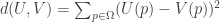
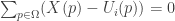
I’ve been talking about all this as if every aspect of utility functions were meaningful. But (as discussed in recent posts) some disagree. Indeed, one very interesting argument for utilitarianism has as a premise that utility functions are invariant under level-changes—i.e the utility function U and the utility function V represent the same underlying desire-state if there is a constant such that for each proposition p, (see Gaertner ch7). Now, it seems like the squared euclidean similarity measure doesn’t jive with this picture at all. After all, if we measure the squared Euclidean distance between U and V that differ by a constant, as above, we get:

On the one hand, on the picture just mentioned, these are supposed to be two representations of the same underlying state (if level-boosts are just a “choice of unit”) and on the other hand, they have positive dissimilarity by the distance measure I’m working with.

Now, as I’ve said in previous posts, I’m not terribly sympathetic to the idea that utility functions represent the same underlying desire-state when they’re related by a level boost. I’m happy to take the verdict of the squared euclidean similarity measure literally. After all, it was only one argument for utilitarianism as a principle of social choice that required the invariance claim–the reverse implication may not hold. In this post we have, in effect, a second independent argument for utilitarianism as a social choice mechanism that starts from a rival, richer preference structure.

But what if you were committed to the level-boosting invariance picture of preferences? Well, really what you should be thinking about in that case is equivalence classes of utility functions, differing from each other solely by a level-boost. What we’d really want, in that case, is a measure of distance or similarity between these classes, that somehow relates to the squared euclidean distance. One way forward is to find a canonical representative of each equivalence class. For example, one could choose the member of a given equivalence class that is closest to the null utility vector–from a given utility function U, you find its null-closest equivalent by subtracting a constant equal to the average utility it assigns to propositions: .

Another way to approach this is to look at the family of squared euclidean distances between level-boosted equivalents of two given utility functions. In general, these distances will take the form

(Where .) You find the minimum element in this set of distances (the closest the two equivalence classes come to each other) by differentiating with respect to gamma and setting the result to zero. That is:

,

which rearranging gives:

Working backwards, set and , and we have defined two level boosted variants of the original U and V which minimize the distance between the classes of which they are representatives (in the square-euclidean sense). But note these level boosted variants are just and . That is: minimal distance (in the square-euclidean sense) between two equivalence classes of utility functions is achieved by looking at the squared euclidean distance between the representatives of those classes that are closest to the null utility.

This is a neat result to have in hand. I think the “minimum distance between two equivalence classes” is better motivated than simply picking arbitrary representatives of the two families, if we want a way of extending the squared-Euclidean measure of similarity to utilities which are assumed to be invariant under level boosts. But this last result shows that we can choose (natural) representatives of the equivalence classes generated and measure the distance between them to the same effect. It also shows us that the social choice compromise which minimizes distance between families of utility can be found by (a) using the original procedure above for finding the utility function selected as a minimum-distance compromise between the reprentative of each family of utility functions; and (b) selecting the family of utility functions that are level boosts of $U_C$. Since the level boosts wash out of the calculation of the relative utilities of a set of options, all the members of the family will agree on which option to choose from a given set.

I want to emphasize again: my own current view is that the complexity intoduced in the last few paragraphs is unnecessary (since my view is that utilities that differ by constant factors from one another represent distanct desire-states). But I think you don’t have to agree with me on this matter to use the minimum distance compromise argument for utilitarian social choice.

Joy is appropriate when you learn that something happens that you *really really* want. Despair is appropriate when you learn that something happens that you *really really* don’t want to happen. Emotional indifference is appropriate when you learn that something happens which you neither want nor don’t want–which is null for you. And there are grades of appropriate emotional responses—from joy to happiness, to neutrality, to sadness, to despair. I take it that we all know the differences in the intensity of the feeling in each case, and have no trouble distinguishing the valence as positive or negative.

More than just level and intensity of desire matters to the appropriateness of an emotional response. You might not feel joy in something you already took for granted, for example. Belief-like as well as desire-like states matter when we assess an overall pattern of belief/desire/emotional states as to whether they “hang together” in an appropriate way–whether they are rationally coherent. But levels and intensities of desire obviously matter (I think).

Suppose you were charged with interpreting a person about whose psychology you knew nothing beforehand. I tell you what they choose out the options facing them in a wide variety of circumstances, in response to varying kinds of evidence. This is a hard task for you, even given the rich data, but if you assumed the personal is rational you could make progress. But if *all* you did was attribute beliefs and desires which (structrurally) rationalize the choices and portray the target as responding rationally to the evidence, then there’d be a distintive kind of in-principle limit built into the task. If you attributed utility and credences which make the target’s choices maximize expected utility, and evolve by conditionalization on evidence, then you’d get a fix on what the target prefers to what, but not, in any objective sense, how much more they prefer one thing to another, or whether they are choosing x over y because x is the “lesser or two evils” or the “greater of two goods”. If you like, think of two characters facing the same situation–an enthusiast who just really likes the way the world is going, but mildly prefers some future developments to others, and the distraught one, who thinks the world has gone to the dogs, but regards some future developments as even worse than others. You can see how the the choice-dispositions of the two given the same evidence could match despite their very different attitudes. So given *only* information about the choice-dispositions of a target, you wouldn’t know whether to interpret the target as an enthusiast or their distraight friend.

While the above gloss is impressionistic, it reflects a deep challenge to the attempt to operationalize or otherwise reduce belief-desire psychology to patterns of choice-behaviour. It receives its fullest formal articulation in the claim that positive affine transformations of a utility function will preserve the “expected utility property”. (Any positive monotone transformation of a utility function will preserve the same ordering over options. The mathetically interesting bit here is that the positive affine transformations of utility function guarantee that the pattern between preferences over outcomes and preferences over acts that bring about those outcomes, mediated by credences in the act-outcome links, are all preserved).

One reaction to this in-principle limitation is to draw the conclusion that really, there are no objective facts about the level of desire we each have in an outcome, or how much more desirable we find one thing than another. A famous consequence of drawing that conclusion is that no objective sense could be made out of questions like: do I desire this pizza slice more or less than you do? Or questions like: does the amount by which I desire the pizza more than the crisps exceed the amount you desire the pizza more than the crisps? And clearly if desires aren’t “interpersonally comparable” in this sort of ways, certain ways of appealing to them within accounts of how its appropriate to trade off one person’s desires against another’s won’t make sense. A Rawlsian might say: if there’s pizza going spare, give it to the person for whom things are going worst (for whom the current situation, pre-pizza, is most undesirable). A utilitarian might say: if everyone is going to get pizza or crisps, and everyone prefers pizza to crisps, give the pizza to the person who’ll appreciate it the most (i.e. prefers pizza over crisps more than anyone else). If the whole idea of interpersonal comparisons of level and differences of desirability are nonsense, however, then those proposals write cheques that the metaphysics of attitudes can’t pay.

(As an aside, it’s worth noting at this point that you could have Rawlsian or utilitarian distribution principles that work with quantities other than desire—some kind of objective “value of the outcome for each person”. It seems to me that if the metaphysics of value underwrites interpersonally comparable quantities like the levels of goodness-for-Sally for pizza, and goodness-difference-between-pizza-and-crisps-for-Harry, then the metaphysics of desires should be such that Sally and Harry’s desire-state will, if tuned in correctly, reflect these levels and differences.)

It’s not only the utilitarian and Rawlsian distribution principles (framed in terms of desires) that have false metaphysical presuppositions if facts about levels and differences in desire are not a thing. Intraindividual ties between intensities of emotional reaction and strength of desire, and between type of emotional reaction and valence of desire, will have false metaphysical presuppositions if facts about an individual’s desire are invariant under affine tranformation. Affine transformations can change the “zero point” on the scale on which we measure desirability, and shrink or grow the differences between desirabilities. But we can’t regard zero-points or strengths of gaps as merely projections of the theorist (“arbitrary choices of unit and scale”) if we’re going to tie to them to real rational constraints on type and intensity of emotional reaction.

However. Suppose in the interpretive scenario I gave you, you knew not only the choice-behaviour of your target in a range of varying evidential situations, but also their emotional responses to the outcome of their acts. Under the same injunction to find a (structurally) rationalizing interpretation of the target, you’d now have much more to go on. When they have emotional reactions rationally linked to indifference, you would attribute a zero-point in the level of desirability. When an outcome is met with joy, and another with mere happiness, you would attribute a difference in desire (of that person, for that outcome) that makes sense of both. Information about emotions, together with an account of the rationality of emotions, allow us to set the scale and unit in interpreting an individual, in a way choice-behaviour alone struggles to. As a byproduct, we would then have a epistemic path to interpersonal comparability of desires. And in fact, this looks like an epistemic path that’s pretty commonly available in typical interpersonal situations–the emotional reactions of others are not *more* difficult to observe than the intentions with which they act or the evidence that is available to them. Emotions, choices and a person’s evidence are all interestingly epistemically problematic, but they are “directly manifestable” in a way that contrasts with the beliefs and desires that mesh with them.

The epistemic path suggests a metaphysical path to grounding levels and relative intensities of desires. Just as you can end up with a metaphysical argument against interpersonal comparability of desires by commiting oneself to grounding facts about desires in patterns of choice-behaviour, and then noting the mathematical limits of that project, you can get, I think, a metaphysical vindication of interpersonal comparabiilty of desire by including in the “base level facts” upon which facts about belief and desire are grounded facts about, type, intensity and valence of intentional emotional states. As a result, the metaphysical presuppositions of the desire-based Rawlsian and utilitarian distribution principles are met, and our desires have the structure necessary to capture and reflect level and valence of any good-for-x facts that might feature in a non-desire based articulation of those kind of principles.

In my book The Metaphysics of Representation I divided the task of grounding intentionality into three parts. First, grounding base-level facts about choice and perceptual evidence (I did this by borrowing from the teleosemantics literature). Then grounding belief-desire intentional facts in the base-level facts, via a broadly Lewisian metaphysical form of radical interpretation. (The third level concerned representational artefacts like words, but needn’t concern us here). In these terms, what I’m contemplating is to add intensional emotional states to the base level, using that to vindicate a richer structure of belief and desire.

Now, this is not the only way to vindicate levels and strength of desires (and their interpersonal comparability) in this kind of framework. I also argue in the book that the content-fixing notion of “correct interpretation” should use a substantive conception of “rationality”. The interpreter should not just select any old structurally-rationalizing interpretation of their target, but will go for the one that makes them closest to an ideal, where the ideal agent responds to their reasons appropriately. If an ideal agent’s strength and levels of desire are aligned, for example, to the strength and level of value-for-the-agent present in a situation, then this gives us a principled way to select between choice-theoretically equivalent interpretations of a target, grounding choices of unit and scale and interpersonal comparisons. I think that’s all good! But I think that including emotional reactions as constraining factors in interpretation can help motivate the hypothesis that there will be facts about the strength and level of desire *of the ideal agent*, and gives a bottom-up data-based constraint on such attributions that complements the top-down substantive-rationality constraint on attributions already present in my picture.

I started thinking about this topic with an introspectively-based conviction that *of course* there are facts about how much I want something, and whether I want it or want it not to happen. I still think all this. But I hope that I’ve now managed to identify how those convinctions to their roles in a wider theoretical edifice–their rational interactions with *obvious* truths about features of our emotional lives, the role of these in distribution principles, which give a fuller sense of what is at stake if we start denying that the metaphysics of attitudes has this rich structure. I can’t see much reason to go against this, *unless* you are in the grip of a certain picture of how attitudes get metaphysically grounded in choice-behaviour. And I like a version of that picture! But I’ve also sketched how the very links to emotional states give you a version of that kind of metaphysical theory that doesn’t have the unwelcome, counterintuitive consequences its often associated with.

How might we measure the proximity or similarity of two belief states? Suppose they are represented in each case as a function from propositions to real numbers between 0 and 1, representing their respective degrees of belief. Is it possible to find a sensible and formally tractable measure of how similar these two states are?

How might we measure the proximity or similarity of two desire states? Suppose they are represented in each case as a function from propositions to real numbers, representing how desirable the agent finds each proposition being true. Is it possible to find a sensible and formally tractable measure of how similar these two states are?

The TL;DR of what follows is: I think we can find a measure of both (or better, a measure of the proximity of pairs of combined belief-desire states). And this idea of proximity between belief-desire psychologies is key to explaining the force of theoretical rationality constraints (probabilism) and means-end practical rationality constraints (causal expected utility theory). Furthermore, it’s the notion we need to articulate the role of “principles of charity” in metasemantics.

The first question above is one that has arisen prominently in accuracy-first formal epistemology. As the name suggests, the starting point of that project is a measure of the accuracy of belief states. Richard Pettigrew glosses the accuracy of a credence function at a world as its “proximity to the ideal credence at that world” (Accuracy and the laws of credence, p.47). If you buy Pettigrew’s main arguments for features of belief-proximity in chapter 4 of this book, then it’s a mathematical consequence that belief-proximity is what’s known as an “additive Bregman divergence”, and if you in addition think that the distance from belief b to belief b* is always the same as the distance from belief b* to belief b (i.e. proximity is symmetric) then one can prove, essentially, that the right way to measure the proximity of belief states Alpha and Beta is by taking the “squared Euclidean distance”, i.e. to take each proposition, take the difference between the real number representing Alpha’s credence in it and that representing Beta’s credence in it, take the square of this difference, and sum up the results over all propositions.

Now, once you have this measure of proximity to play with, accuracy-firsters like Pettigrew can put it to work in their arguments for the rational constraints on belief. Accuracy of a belief in w is proximity to the ideal belief state in w; if the ideal belief state for an agent x in w is one that matches the truth values of each proposition (“veritism”) then one can extract from the measure of proximity a measure of accuracy, and go on to prove, for example, that a non-probabilistic belief state b will be “accuracy dominated”, i.e. there will be some alternative belief state b* which is *necessarily* more accurate than it.

So far, so familiar. I like this way of relating theoretical rational constraints like probabilism to what’s ultimately valuable in belief–truth. But I’m also interested in notion of proximity for other reasons. In particular, when working in metasemantics, I want to think about principles of interpretation that take the following shape:

(I) On the basis of the interpreter’s knowledge of some primary data, and given constraints that tie possible belief states to features of that primary data, the interpreter is in a position to know that the target of interpretation has a belief state within a set C.

(II) The interpreter attributes to the target of interpretation that belief state within C which is closest to belief state m.

To fix ideas: the set C in (I) might arise out of a process of finding a probability-utility pair which rationalizes the target’s choice behaviour (i.e. always makes the option the target chooses the one which maximizes expected utility, by their lights, among the options they choose between). The magnetic belief state “m” in (II) might be the ideal belief state to have, by the interpreter’s lights, given what they know about the target’s evidential setting. Or it might be the belief state the interpreter would have in the target’s evidential setting.

There are lots of refinements we might want to add (allowing m to be non-unique, catering for situations in which there are several elements in C that are tied for closeness to m). We might want to clarify whether (I) and (II) are principles of practical interpretation, somehow mapping the processes or proper outputs of a real-life flesh and blood interpreter, or whether this is intended as a bit of theory of ideal interpretation, carried out on the basis of total “knowledge” of primary facts about the target. But I’ll set all that aside.

The thing I want to highlight is that step (II) of the process above makes essential use of a proximity measure. And it’s pretty plausible that we’re here shopping in the same aisle as the accuracy-first theorists. After all, a truth-maximizing conception of principles of interpretation would naturally want to construe (II) as attributing to the subject the most accurate belief state within the set C, and we’ll get that if we set the “ideal” credence (in a given world) to be the credal state that matches the truth values at that world, in line with Pettigrew’s veritism, and understand proximity in the way Pettigrew encourages us to. Pettigrew in fact defends his characterization of proximity independently of any particular identification of what the ideal credences are. If you were convinced by Pettigrew’s discussion, then even if the “ideal credence” m for the purposes of interpretation is different from the “ideal credence” for the purposes of the most fundamental doxastic evaluation, you’ll still think that the measure of proximity—additive Bregman divergence/squared Euclidean distance–is relevant in both cases.

That’s the end of the (present) discussion as far as belief goes. I want to turn to an extension to this picture that becomes pressing when we think of this in the context of principles of interpretation. For in the implementations that I am most interested in, what we get out of step (I) is not a set of belief states alone, but a set of belief-desire psychologies—a pairing of credence and utility functions, for example. Now, it’s possible that the second step of interpretation, (II), cares only about what goes on with belief—picking the belief-desire psychologies whose belief component is closest to the truth, to the evidence, or to the belief state component of some other relevantly magnetic psychological state. But the more natural version of this picture wouldn’t simply forget about the desires that are also being attributed. And if it is proximity between belief-desire psychologies in C and magnetic belief-desire psychology m that is at issue, we are appealing to a proximity not between belief states alone, but proximity between pairs of belief-desire states.

If desire states are represented by a function from propositions to real numbers (degrees of desirability) then there’s clearly a straight formal extension of the above method available to us. If we used squared euclidean distance as a measure of the proximity or similarity of a pair of belief states, use exactly the same formula for measuring the proximity of similarity of desire! But Pettigrew’s arguments for the characteristics which select that measure do not all go over. In particular, Pettgrew’s most extended discussion is in defence of a “decomposition” assumption that makes essential use of notions (e.g. “well-calibrated counterpart of the belief state”) that do not have any obvious analogue for belief-desire psychologies.

Is there anything to be said for the squared euclidean distance measure of proximity between belief-desire psychologies, in the absence of an analogue of what Pettigrew says in the special case of proximity of belief states? Well, one thing we can note is that as it extends Pettigrew’s measure of the proximity of belief states, it’s consistent with it–a straight generalization is the natural first hypothesis for belief-desire proximity to try, relative to the Pettigrew starting point. What I want to now discuss is a way of getting indirect support for it. What I’ll argue is that it can do work for us analogous to the work that it does for the probabilist in accuracy framework.

To get the inaccuracy framework off the ground, recall, Pettigrew commits to the identification of an ideal belief state at each world. The ideal belief state at w is that belief state whose levels of confidence in each proposition matches the truth value of that proposition at w (1 if the proposition is true, 0 if the proposition is false). To add something similar for desire, instead of truth values, let’s start from a fundamental value function defined over the worlds, V, measured by a real number. You can think of the fundamental valuation relation as fixed objectively (the objective goodness of the world in question), fixed objectively relative to an agent (the objective goodness of the world for that agent), as a projection of values embraced by the particular agent, or some kind of mix of the above. Pick your favourite and we’ll move on.

I say: the ideal degree of desirability for our agent to attach to the proposition that w is the case is V(w). But what is the ideal degree of desirability for other, less committal propositions? Here’s a very natural thought (I’ll come back to alternatives later): look at which world would come about were p the case, and the ideal desirability of p is just V(w) for that w which p counterfactually implies. (This, by the way, is a proposal that makes heavy reliance on the Stalnakerian idea that for every world there is a unique closest world where p). So we extend V(w), defined over worlds, to V*(p), defined over propositions, via counterfactual connections of this kind.

If we have this conception of ideal desires, and also the squared-euclidean measure of proximity between desire states, then a notion of “distance from the ideal desire state” drops out. Call this measure the misalignment of a desire state. If we have the squared-euclidean masure of proximity between combined belief-desire states, then what drops out is a notion of “distance from the ideal belief-desire state”, which is simply the sum of the inaccuracy of its belief component and the misalignment of its desire component.

The fundamental result that accuracy-firsters point to as a vindication of probabilism is this: unless a belief state b is a convex combination of truth values (i.e. a probability function) then there will be a b* which is necessarily more accurate than b. In this setting, the same underlying result (as far as I kind see—there are a few nice details about finitude and boundedness to sort out) delivers this: unless belief-desire state <b,d> is a convex combination over w of vectors of the form <truth-value at w, V-value at w>, then will be some alternative psychology <b*,d*> which will necessarily be closer to the ideal psychology (more accurate-and-aligned) than is <b,d>.

What must undominated belief-desire psychologies be like? We know they must be convex combinations of <truth value at w, V-value at w> pairs for varying w. The b component will then be a convex combination of truth values with weights k(w), i.e. a probability function that invests credence k(w) in w. More generally, both the b and d components are expectations of random variables with weights k(w). b(p) will be the expectation of indicator random variables for proposition p, and d(p) the expectation of the value-of-p random variable. The expectation of the value-of-p random variable turns out to be equal to the sum over all possible values of k of the following: k multiplied by the agent’s degree of belief of the counterfactual conditional if p had been the case, then value of the world would be k. And that, in effect, is Gibbard-Harper’s version of causal decision theory.

If the sketch above is correct, then measuring proximity of whole psychologies by squared euclidean distance (or more generally, an additive Bregman divergence), will afford a combined accuracy-domination argument for probabilism and value-domination argument for causal decision theory. That’s nice!

Notice that there’s some obvious modularity in the argument. I already noted that we could treat V(w) as objective, relativized or subjective value. Further, we get the particular Gibbard-Harper form of causal decision theory because we extended the ideal V over worlds to ideal V* over propositions via counterfactual conditionals concerning which world would obtain if p were the case. If instead defined the ideal V* in p as the weighted average of the values of worlds, weighted by the conditional chance of that world obtaining given p, then we’d end up with an expected-chance formulation of causal decision theory. If we defined the ideal V* in p via combinations of counterfactuals about chance, we would derive a Lewisian formulation of causal decision theory. If we reinterpret the conditional in the formulation given above as an indicative conditional, then we get a variant of evidential decision theory, coinciding with Jeffrey’s expected decision theory only if the probability of the relevant conditional is always equal to the corresponding conditional probability (that thesis, though, is famously problematic).

Okay, so let’s sum up. What has happened here is that, for the purposes of formulating a particular kind of metasemantics of belief and desire, we need a notion of proximity of whole belief-desire psychologies for one another. Now, Pettigrew has explicitly argued for specific way of measuring proximity for the belief side of the psychology. The natural thing to do is to extend his arguments to descriptions of psychological states including desires as well as beliefs. But unfortunately, his arguments for that specific way of handling proximity look too tied to belief. However, we can provide a more indirect abductive argument for the straight generalization of this way of measuring proxmity over belief-desire psychologies by (a) endorsing Pettigrew’s arguments for the special case of belief; and (b) noting that the straight generalization of this would provide a uniform vindication of both probabilism and standard rational requirements on desire as well as belief.

This, at least, makes me feel that I should be pretty comfortable at appealing to a notion of “proximity to the magnetic belief-desire state m” in formulating metasemantics in the style above, and measuring this by squared Euclidean distance—at least insofar as I am bought in to the conception of accuracy that Pettigrew sketches.

Let me make one final note. I’ve been talking throughout as if we all understood what real-valued “degrees of desire” are. And the truth is, I believe I do understand this. I think that I have neutral desire for some worlds/propositions, positive desire for others, negative for a third. I think that we can measure and compare the gap between the desirability of two propositions—the difference between the desirability of eating cake and eating mud is much greater than the difference between the the desirability of overnight oats and porridge. I think there are facts of the matter about whether you and I desire the same proposition equally, or whether I desire it more than you, or you desire it more than me.

But famously, some are baffled by interpersonal comparisons of utility, or features of the utility-scale, of the kind I instinctively like. If you think of attributing utility as all about finding representations that vindicate choice behaviour, interpersonal comparisons will be as weird as the idea of an interpersonal choice. The whole project of measuring proximity between desireability states via functions on their representations as real values might look like a weird starting point. If you google the literature on similarity measures for utility, you’ll find a lot of work on similarity of preference orderings e.g. by counting how many reversals of the orderings it takes to turn one into another. You might think this is a much less controversial starting point than what I’m doing, and that I need to do a whole heap more work to earn the right to my starting point.

I think the boot is on the other foot. The mental metasemantics in which I aim to deploy this notion of proximity denies that all there is to attributing utility is to find a representation that vindicates the agent’s choice behaviour. That’s step I, but step II goes beyond this to play favourites among the set of vindicatory psychological states. By the same token, the mental metasemantics sketched grounds interpersonal comparisons of desirability between various agents, by way of facts about the proximity of the desirability of the agent’s psychology to the magnetic psychological state m.

There’s a kind of dialectical stalemate here. If interpersonal comparisons are a busted flush, the prospects look dim for any kind of proximity measure of the kind I’m after here (i.e. one that extends the proximity implicit in accuracy-first framework). If however, the kind of proximity measures I’ve been discussing make sense, then we can use them to ground the real-value representations of agent’s psychological states that make possible interpersonal comparisons. I don’t think either myself or my more traditional operationalizing opponent here should be throwing shade at the other at this stage of development–rather, each should be allowed develop their overall account of rational psychology, and at the end of the process we an come back and compare notes about whose starting assumptions were ultimately more fruitful.

The TL;DR summary of what follows is that we should quantify the conventionality of a regularity (David-Lewis-style) as follows:

A regularity R in the behaviour of population P in a recurring situation S, is a convention of depth x, breadth y and degree z when there is a recurring situation T that refines S, and in each instance of T there is a subpopulation K of P, such that it’s true and common knowledge among K in that instance that:

(A) BEHAVIOUR CONDITION: everyone in K conforms to R
(B) EXPECTATION CONDITION: everyone in K expects everyone else in K to conform to R
(C) SPECIAL PREFERENCE CONDITION: everyone in K prefers that they conform to R conditionally on everyone else in K conforming to R. 

where x (depth) is the fraction of S-situations which are T, y (breadth) is the fraction of all Ps involved who are Ks in this instance, and z is the degree to which (A-C) obtaining resembles a coordination equilibrium that solves a coordination problem among the Ks.

From grades of conventionality so defined, we can characterize in the obvious way a partial ordering of regularities by whether one is more of a convention than another. What I have set out differs in several respects from what Lewis himself proposed along these lines. The rest of the post spells out why.

The first thing to note is that in Convention Lewis revises and re-revises what it takes to be a convention. The above partial version is a generalization of his early formulations in the book. Here’s a version of his original:

A regularity R in the behaviour of a population P in a recurring situation S is a convention if and only it is true that, and common knowledge in P that:

(A) BEHAVIOUR CONDITION: everyone conforms to R
(B) EXPECTATION CONDITION: everyone expects everyone else to conform to R
(C) SPECIAL PREFERENCE CONDITION: everyone prefers that they conform to R conditionally on everyone else conforming to R. 

where (C) holds because S is a coordination problem and uniform conformity to R is a coordination equilibrium in S.

A clarificatory note: in some conventions (e.g. a group of friends meeting in the same place week after week) the population in question are all present in instances of the recurring situation. But in others—languages, road driving conventions—the recurring situation involves more or less arbitrary selection of pairs, triples, etc of indiviuduals from a far larger situation. When we read the clauses, the intended reading is that the quantifiers “everyone” be restricted just to those members of the population who are present in the relevant instance of the recurring situation. The condition is then that it’s common knowledge instance-by-instance *between conversational participants* or *between a pair of drivers* what they’ll do, what they expect, what they prefer, and so on. That matters! For example, it might be that strictly there is no common knowledge at all among *everyone on the road* about what side of the road to drive on. I may be completely confident that there’s at least one person within the next 200 miles not following the relevant regularity. Still, I may share common knowledge with each individual I encounter, that in this local situation we are going to conform, that we have the psychological states backing that up, etc. (For Lewis’s discussion of this, see his discussion of generality “in sensu diviso” over instances). 

Let me now tell the story about how Lewis’s own proposal arose. First, we need to see his penultimate characterization of a convention:

A regularity R in the behaviour of P in a recurring state S, is a perfect convention when it’s common knowledge among P in any instance of S that:

(A) BEHAVIOUR CONDITION: everyone conforms to R
(B) EXPECTATION CONDITION: everyone expects everyone else to conform to R
(C) SPECIAL PREFERENCE CONDITION: everyone prefers that they conform to R conditionally on everyone else conforming to R. 
(D) GENERAL PREFERENCE CONDITION: everyone prefers that anyone conform to R conditionally on all but one conform to R.
(E) COOPERATION CONDITION: everyone has approximately the same preferences regarding all possible combinations of actions
(F) There exists an alternative regularity R* incompatible with R, which also meets the analogue of (C) and (D). 

The explicit appeal to coordination problems and their solution by coordination equilibria has disappeared. Replacing them are the three clauses (D-F). In (D) and (E) Lewis ensures that the scenario resembles recurring games of pure cooperation in a two specific, independent respects. Games of pure cooperation have exact match of preferences over all possible combinations of outcomes (cf. (E)’s approximate match). And because of this perfect match, if any one person prefers to conform conditionally on others conforming, all others share that preference too (cf (D)). So by requiring (D) we preserve a structural feature of coordination problems, and by requiring (C) we require some kind of approximation to a coordination problem. (F) on the other hand is a generalization of the condition that these games have more than one “solution” in the technical sense, and so are coordination *problems*.

It’s striking that, as far as I can see, Lewis says nothing about what further explanatory significance (beyond being analytic of David Lewis’s concept of convention) these three features enjoy. That contrasts with the explanatory power of (A-C) being true and common knowledge, which is at the heart of the idea of a rationally self-sustaining regularity in behaviour. I think it’s well worth keeping (A-C) and (D-F) separate in one’s mind when thinking through these matters, if only for this reason.

Here’s the Lewisian proposal to measure degree of conventionality:

A regularity R in the behaviour of P in a recurring situation S, is a convention to at least degree <z,a,b,c,d,e,f> when it’s common knowledge among P in at least fraction z of instances of S that:

(A*) BEHAVIOUR CONDITION: everyone in some fraction a of P conforms to R
(B*) EXPECTATION CONDITION: everyone in some fraction b of P expects a fraction of at least a of P else to conform to R
(C*) SPECIAL PREFERENCE CONDITION: everyone in some fraction c of P prefers that they conform to R conditionally on everyone in fraction a of P conforming to R. 
(D*) GENERAL PREFERENCE CONDITION: everyone in some fraction d of P prefers that anyone conform to R conditionally on everyone in fraction a of P conforming to R.
(E*) COOPERATION CONDITION: everyone on some fraction e of P has approximately the same preferences regarding all possible combinations of actions
(F*) there exists an alternative regularity R* incompatible with R in fraction f of cases, which also meets the analogue of (C) and (D). 

The degree of conventionality of R is then defined to be the set of tuples such that R is a convention to degree at least that tuple. A partial order of comparative conventionality can then be defined in the obvious way.

While measuring the degree to which the clauses of the characterization of perfect conventionality are met is a natural idea, there’s just no guarantee that it tracks anything we might want from a notion of partial conventionality, e.g. “resemblance to a perfect convention”. I’ll divide my remarks into two clusters: first on (A-C), and then on (D-F).

One the original conception, the (A-C) clauses work together in order to explain what a convention explains. That’s why, after all, Lewis makes sure that in clause C* the conditional preference is condition on the obtaining of the very fraction mentioned in clause (A*) and (B*). But more than this is required.

On that original conception, the rationality of conformity to (A) is to be explained by (common knowledge of) the expectations and preferences in (B) and (C). Where everyone has the expectations and preferences, the rationalization story roles along nicely. But once we allow exceptions, things break down.

Consider, first, the limit case where nobody at all has the expectation or preference (so (B,C) are met to degree zero). A regularity in conforming to the regularity can then be entirely accidental, obtaining independently of the attitudes prevailing among those conforming. Such situations lack the defining charactistics of a convention. But (holding other factors equal) Lewis’s definition orders them by how many people in the situation conform to the regularity. So, Lewis finds an ordering where this is really none to be had. That’s bad.

Consider, second, a case where the population divides evenly into two parts: those who have the preference but no expectation, and those who have the expectation but no preference. No person in any instance will have both the expectation and preference that in the paradigm cases work together to rationality support the regularity. To build a counterexample to Lewis’s analysis of comparative conventionality out of this, consider a situation where the expectation and preference clause are met to degree 0.4, but by the same group, which rationalizes 0.4 conformity. Now we have a situation where expectations and preferences do sustain the level of conformity, and so (all else equal) it deserves to be called a partial convention. But on Lewis’s characterization it is less of a convention than a situation where 50% of people have the preference, a non-overlapping 50% have the expectation, and 40% irrationally conform to the regularity. The correct view is that the former regularity is more conventional than the latter. Lewis says the opposite. I conclude Lewis characterized the notion of degree of convention in the wrong way. 

Let me turn to the way he handles (D-F). What’s going on here, I think, is that he’s picking up three specific ways in which what’s going on can resemble a solution to a coordination problem. But there are again multiple problems. For a start, there are the kind of lack-of-overlap problems we just saw above. A situation where 40% of the people conform, and meet the relevant expectations and preference clause, and perfectly match in preferences over all relevant situations, is ranked *below* situations where 40% of people conform, meet the relevant expectations and preference clause, and are completely diverse in their preferences *but* the remaining 60% of the population has perfectly matched preferences against conformity to R. That’s no good at all!

But as well as the considerations about overlap, the details of the respects of similarity seem to me suspect. For example, consider a scenario where (A-C) are fully met, and everybody has preferences that diverge just too much to count as approximately the same, so (E) is met to degree zero. And compare that to a situation where two people have approximately the same preferences, and 98 others have completely divergent preferences. Then (E) is met to degree 0.02. The first is much more similar to perfect match of preferences than the second, but Lewis’s ranking gives the opposite verdict. (This reflects the weird feature that he loosens the clause from exact match to approximate match, and then on *top* of that loosening, imposes a measure of degree of satisfaction. I really think that the right thing here is to stick with a measure of similarity of preference among a relevant group of people, rather than counting pairwise exact match).

I’d fold in clause F into the discussion at this point, but my main concerns about it would really turn into concerns about whether Lewis’s model of conventions as equilibria is right, and that’d take me too far afield. So I’ll pass over it in silence.

To summarize. Lewis’s characterization of degrees of conventionality looks like it misfires a lot. The most important thing wrong with it that it doesn’t impose any sort of requirement that its clauses to be simultaneously satisfied. And that leaves it open to the kind of problems below.

My own proposal, which I listed at the start of this post, seems to me to be the natural way to fix this problem. I say: what we need to do is look for “kernals” of self-sustaining subpopulations, where we insist that each member of the kernal meets the conformity, expectation and preference conditions perfectly. The size of this kernal, as a fraction of those in the population involved in the situation, then measures how closely we approximate the original case. That fraction I called the “depth” of the convention, where a convention with depth 1 involves everyone involved in any instance of the situation pulling their weight, and a convention with depth 0.5 being one where only half are involved, but where that is still just as rationally self-sustaining as a case of perfect convention. We might introduce the neologism “depth of subconvention” to articulate this:

A regularity R in the behaviour of P in a recurring situation S, is a sub-convention of depth x when in every instance of S there is kernal K of the members of P such that it’s true and common knowledge among K in this instance of S that:

(A**) BEHAVIOUR CONDITION: everyone in K conforms to R
(B**) EXPECTATION CONDITION: everyone in K expects everyone in K to conform to R
(C**) SPECIAL PREFERENCE CONDITION: everyone in K prefers that they conform to R conditionally on everyone in K conforming to R. 

and x is the fraction of P in the instance of S who are in K.

(These clauses contain a free variable K embedded in specifications of preference and expectation. So what is the content of the preferences and the expectations we’re here requiring? Do the people in the kernal satisfying the conditions need to conceive of the others in K who they expect to conform as being large enough (size k?) Or is it enough that they form preferences and expectations about a subgroup of those involved in the present instance, where that subgroup happens to be of size k? I go with the former, more liberal understanding. In cases where participants interests are grounded in the kind of success that requires k people to cooperate, then (C**) will likely not be met unless all participants have the belief that there are at least k of them. But that isn’t written into the clauses—and I don’t think it should be. Size might matter, but there’s no reason to think it always matters.)

To see why “breadth” as well as “depth” matters, consider the following setup. Suppose that our overall population P divides into conformers C (90%) and the defectors D (10%). The conformers are such that in any instance of S they will satisfy (A-C), whereas the defectors never do (for simplicity, suppose they violate all three conditions). So, if you’re a conformer, you always conform to R whenever you’re in S, because you prefer to do so if 90% of the others in that situation do, and you expect at least 90% of them to do so. 

If everyone in P is present in each instance of S, this will be a straightforward instance of a partial subconvention, to degree 0.9. The biggest kernal witnessing the truth of the above clauses is simply the set of conformers, who are all present in every case.

But now consider a variantion where not all members of P are present in every case. Stipulate that the members of P present in a given instance of S are drawn randomly from the population as a whole. This will not be a partial convention to degree 0.9. That is because there will be instances of S where by chance, too many defectors are present, and the set of conformers is less than the fraction 0.9 of the total involved in that situation. So the set of conformers present in a given instance is sometimes but not always a “kernal” that meets the conditions laid down. Indeed, it is not a convention to any positive degree, because it could randomly be that only defectors are selected for an instance of S, and in that instance there is no kernal of size >0 satisfying the clauses. So by the above definition it won’t be a partial convention to any positive degree, even if such instances are exceptionally rare. 

What we need to avoid this is to provide for exceptions to the “breadth” of the convention, i.e. the instances of S where the clauses are met, as Lewis does:

A regularity R in the behaviour of population P in a recurring situation S, is a convention of depth x, breadth y when there is a recurring situation T that refines S, and in each instance of T there is a subpopulation K of P, such that it’s true and common knowledge among K in that instance that:

(A**) BEHAVIOUR CONDITION: everyone in K conforms to R
(B**) EXPECTATION CONDITION: everyone in K expects everyone in K to conform to R
(C**) SPECIAL PREFERENCE CONDITION: everyone in K prefers that they conform to R conditionally on everyone in K conforming to R

and x is the fraction of S situations that are T situations and y is the fraction of P in the instance of T that are in K.

(I’ve written this in terms of a new recurring state T, rather than (per Lewis) talking about a fraction of the original recurring state type, to bring out the following feature. In the special case I’ve been discussing, where the largest kernal witnessing the truth of these clauses is simply those conformers present in C, then when the clauses are met with depth x and breadth y with respect to S and P, they will be met with depth 1 and breadth 1 with respect to T and C. That is: in this special case, the clauses in effect require there be a perfect subconvention with respect to some subpopulation and substitution of the population and situation we start from. Depth and Breadth of subconventionality is then measuring the fraction of the overall population and state that these “occupy”.

What do we now think about the remaining clauses of Lewis’s definition? I think there’s no obvious motive for extending the strategy I’ve pursued to this point, of requiring these clauses be satisfied perfectly by the kernal K. After all, (common knowledge of) the satisfaction of (A-C) already provides for the rational stability of the pattern of conformity. But equally (as we saw in one of my earlier objections to Lewis) we don’t want to measure the fraction of all those involved in the recurring situation who satisfy the clauses, else we’ll be back to problems of lack of overlap. What we want to do is take the kernal we have secured from subconvention conditions already set down, and look at the characteristics of the regularity that prevails among them. To what extent is that rationally stable regularity a convention? And that brings us right up to my official proposal, repeated here:

A regularity R in the behaviour of population P in a recurring situation S, is a convention of depth x, breadth y and degree z when there is a recurring situation T that refines S, and in each instance of T there is a subpopulation K of P, such that it’s true and common knowledge among K in that instance that:

(A) BEHAVIOUR CONDITION: everyone in K conforms to R
(B) EXPECTATION CONDITION: everyone in K expects everyone else in K to conform to R
(C) SPECIAL PREFERENCE CONDITION: everyone in K prefers that they conform to R conditionally on everyone else in K conforming to R. 

where x (depth) is the fraction of S-situations which are T, y (breadth) is the fraction of all Ps involved who are Ks in this instance, and z is the degree to which (A-C) obtaining resembles a coordination equilibrium that solves a coordination problem among the Ks.

The key thing to note here, compared to the previous version, is that I’ve declined to unpack the notion of “resembling a coordination equilibrium that solves a coordination problem”. For all that’s been said here, you could look at the implicit analysis that Lewis’s (D*-E*) gives of this notion (now restricted to the members of the kernal), and plug that in. But earlier I objected to that characterization–it doesn’t seem to me to that the fraction of people with approximately matching preferences is a good measure of similarity to the original. In the absence of a plausible analysis, better to keep the notion as a working primitive (and if it doesn’t do much explanatory work, as is my current working hypothesis, analyzing that working primitive will be low down the list of priorities).

A closing remark. Lewis’s official position is neither the unrestricted (A-F) nor the quantative (A*-F*) above. Rather, he gives a version of (A-F) in which quantifiers throughout are replaced by ones that allow for exceptions (“almost everyone…”). But as far as I can see, the same kinds of worries arise for this case—for example, given any threshold for how many count as “almost everyone”, almost everyone can have the relevant conditional preference, almost everyone can have the relevant expectation, but it be not the case that almost everyone have both the preference and expectation, and so if almost everyone conforms to a regularity, at least some of that conformity is not rationalized by the attitudes guaranteed by the other clauses. To fix this, we can extract a “threshold” variant from the quantative proposal I have proposed, which would look like this:

A regularity R in the behaviour of population P in a recurring situation S, is a convention when there is a recurring situation T that refines S, and in each instance of T there is a subpopulation K of P, such that it’s true and common knowledge among K in that instance that:

(A) BEHAVIOUR CONDITION: everyone in K conforms to R
(B) EXPECTATION CONDITION: everyone in K expects everyone else in K to conform to R
(C) SPECIAL PREFERENCE CONDITION: everyone in K prefers that they conform to R conditionally on everyone else in K conforming to R. 

where almost all S-situations are T, almost all P involved in the instance of T are in K, and (A-C) obtaining is almost a coordination equilibrium that solves a coordination problem among the Ks.

Here “almost a coordination equilibrium” is to be read as “having a high enough degree of similarity to a coordination equilibrium”.

If you believe p, do you believe you believe p?

Here’s one model for thinking about this. You have the first order belief—you believe p. On top of that, you have some extra mechanism (call it doxastic introspection) that monitors your internal state and extracts information about what beliefs you have. If that extra mechanism is working reliably in this instance, you’ll end up with the (true) belief that you believe p.

On the introspective model, it’s easy to see how first and second order beliefs can get out of alignment. One forms the first order belief, and the extra mechanism for some reason doesn’t work (maybe it’s unreliable in edge cases, and this is an edge case of having a first order belief). So you end up with the false belief that you don’t believe p, or (more modestly, suspending judgement on the issue). Only if we had a magical 100% reliable intrspective mechanism should we expect the original conditional to be always true.

There’s a rival way of thinking about this: the entailment model. On this model, the basic doxastic attitude is not belief, but a propositional attitude we can call “taking for granted”. Whenever you take p for granted in the relevant sense, it automatically follows that you believe p; and it also follows that you believe that you believe p, and so on. So long as the only way humans get to believe p is by taking p for granted, it’ll follow that whenever you believe p, you believe that you believe p. So the original conditional is always true, and not by any magical flawless introspective mechanism, but a “common cause” psychological structure that ensures the first order and higher order belief are formed together.

(Compatibly with this, it might be the case that sometimes you believe you believe p, even though you don’t believe p. After all, there’s nothing in the entailment model that guarantees that when you don’t believe p, you believe you don’t believe p. You’d get that additional result if you added to the assumptions above that the only way humans have of forming the higher order belief that they believe p is by taking p for granted. But as things stand, the entailment model allows that your most basic attitude can be: taking for granted that one believes that p. And that doesn’t itself require you to believe that p).

What might “taking for granted” be, such that the entailment relations mentioned above hold? Here I’m taking a leaf out of work I’ve been doing on common knowledge and public information. There, I’ve been starting from a psychological attitude I’ve called “taking for granted among a group G” (or “treating as public among G”). The idea is that things we take for granted among a group are things we hold fixed in deliberation even when simulating other group member’s perspectives. So, for example, I might see a car about to pull out in front of you from a side street, but also see that you can’t see the car. In one sense, I hold fixed in my own deliberation about what to do next that the car is about to pull out. But I do not hold that proposition fixed in the stronger sense, because in simulating your perspective (and so expected choices) in the next few seconds, most of the scenarios involve no car pulling out. On the other hand, that drivers will slam the breaks when they see a new obstacle in their way, that things fall downward when dropped, that every driver wants to avoid crashes–these are all things I hold fixed in simulating any relevant perspective. They are things that I take for granted among the group consisting of me and you. What I take for granted between us has an important role in rationalizing my actions in situations of interdependent decision.

It’s plausible that x taking-p-for-granted among G entails (i) x believes p (since they hold p fixed in their own deliberation); (ii) x believes that all Gs believe p (since they hold p fixed in their simulations of other group-member’s deliberations). Further iterations also follow. I’ve got work elsewhere that lays out a bunch of minimal conditions on this attitude which deliver the result: for x to take-p-for-granted among G is for x to believe that it is commonly believed that p (where common belief is understood as the standard infinite conjunction of iterated higher order belief conditions).

But consider now the limiting singleton case, where x takes-p-for-granted among the group {x}. Following the pattern above, that requires inter alia that (i) x believes p; (ii) x believes that everyone in {x} believes p. The latter is equivalent to: x believes that x believes p. So this primitive attitude of taking for granted, in the strong sense relevant to group deliberation, has as its limiting singleton case an attitude which satisfies the conditions of the entailment model.

Now, it’s a contingent matter whether human psychology contains an attitude like taking-p-for-granted-among-G. But suppose it does do so. Then it would seem otiose for it to contain an additional primitive attitude of first-order belief, when the limiting de se singleton case of taking-for-granted-among-{x} could do the job. Now, it does the job by way of an attitude that is more committal than belief, in one sense. Taking-p-for-granted is correctly held only when p, plus the world meet some logically independent condition q (which includes that one believes that p). But crucially, these extra conditions on taking-for-granted are self-vindicating. When one takes-for-granted among {oneself} that p, then one can go wrong if not-p. But one cannot go wrong by it failing to be the case that one doesn’t believe p, because ex hypothesi, taking p for granted entails believing p. And this goes for all the extra conditions that it takes for taking-for-granted to be correct that go beyond what it takes for believing-p to be correct. So even though “taking for granted” is stronger than belief, it’s no riskier.

On this model of human psychology rather than having to deal with an array of primitive attitudes with metacognitive contents (I believe that p, I believe that I believe that p, etc), we work with attitudes with simple first-order content, but which have an internal functional role which does the work for which you’d otherwise need metacognitive content. There can then be, in addition, really genuine cases of basic attitudes with true metacognitive content (as when I take for granted that I believe p, but do not take for granted p). And there may be specialized situations where that true metacognitive thinking is necessary or helpful. But for the general run of things, we’ll get by with first-order content alone.

Why might we hestitate to go with the entailment model? Well, if we had clear counterinstances to the original conditional, we’d need to be able to describe how they arise. And counterinstances do seem possible. Someone might, for example, accept bets about how they will act in the future (e.g. bet that they’d pick up the right hand box in an attempt to get cake) but when the moment comes, acts in another way (e.g. choose the left hand box). The final behaviour is in line with a belief that there’s cake in the right hand box; the earlier betting behaviour is in line with the agent failing to believe that they believe there’s cake in that box (it is in line, instead, with a belief that they believe there’s cake in the other box).

Now these kind of cases are easily explained by the introspection model as cases where the introspective mechanism misfires. Indeed, that model esssentially posits a special purpose mechanism plugging away in all the normal ways, just so we can say this about the recherche cases where first and higher order beliefs seem to come apart. What can the friend of the entailment model say about this?

There are two strategies here.

One is to appeal to “fragmentation”. The person concerned has a fragmented mind, one of which includes a taking-for-granted-p, and the other of which doesn’t (and instead includes a taking-for-granted-I-believe-p, or perhaps even a taking-for-granted-not-p). The fragments are dominant in different practical situations. If one already thinks that fragments indexed to distinct practical situations is part of what we need to model minds, then it’s no new cost to deploy the resources to make for the kind of case just sketched. By contrast to the introspective model, we don’t have any special machinery functioning in the normal run of cases, but rather a special (but independently motivated) phenomenon arising which accounts for what happens in the rare cases where first and higher order belief comes apart.

Another strategy that’s available is to loosen the earlier assumption that the only way that humans believe p is via taking p for granted. One insists that this is the typical way that humans believe p (and so, typically, when one believes p that’s because one takes p for granted, and hence believes one believes p too). But one allows that there are also states of “pure” believing-that-p, which match only the first-order functional role of taking for granted. (Compare: most of us think there are acceptance-states other than belief–pretense, say–which are like belief in many ways, but where acceptance-that-p is tied to acting-as-if-p only for a restricted range of contexts. Just so, on this account pure belief will be an artificially restricted version of the taking-for-granted, not the usual stock in trade of our cognitive processing, but something which can get into if the need demands, or lapse into as the result of unusual circumstances).

(I don’t want to pin anybody else with either of these models. But I should say that when I’m thinking about the entailment model, I have in mind certain things that Stalnaker says in defence of principles like the conditional from which I start—the idea that believing you believe p when you believe p is the default case, and that it failures of that tie that require justification, not the other way around.)

To a first approximation, decision theoretic representation theorems take a bunch of information about (coherent) choices of an agent x, and spit out probability-utility pairs that (structurally) rationalize each of those choices. Call that the agential candidates for x’s psychology.

Problems arise if there are too many agential candidates for x’s psychology—if we cannot, for example, rule out hypotheses where x believes that the world beyond her immediate vicinity is all void, and where her basic desires solely concern the distribution of properties in that immediate bubble. And I’ve argued in other work that we do get bubble-and-void problems like these.

I also argued in that work that you could resolve some of the resulting underdetermination by appealing to substantive, rather than structural rationality. In particular, I said we make a person more substantively rational by representing her IBE inferences by inferences to genuinely good explanations (like the continued existence of things when they leave her immediate vicinity) than some odd bubble-and-void surrogate.

So can we get a simple model for this? One option is the following. Suppose there are some “ideal priors” that encode all the good forms of inference to the best explanation . And suppose we’re given total information about the total evidence available to x (just as we were given total information about her choice-dispositions). Then we can construct an ideal posterior probability, , which are the ideal doxastic attitudes to have in x’s evidential situation. Now, we can’t simply assume that x is epistemically ideal–there’s no guarantee that there’s any probability-utility pair among the agential candidates for x’s psychology whose first element matches . But if we spot ourselves a metric of closeness between probability functions, we can consider the following way of narrowing down the choice-theoretic indeterminacy: the evidential-and-agential candidates for x’s psychology will be those agential candidates for x’s psychology whose first component is maximally close to the probability function .

(One warning about the closeness metric we need—I think you’ll get the wrong results if this were simply a matter of measuring the point-wise similarity of attitudes. Roughly—if you can trace the doxastic differences between two belief states to a single goof that one agent made that the other didn’t, those can be similar even if there are lots of resulting divergences. And a belief state which diverged in many different unrelated ways—but where the resulting differences are less far reaching—should in the relevant sense be less similar to one of the originals than either is from each other. A candidate example: the mashed up state which agrees with both where they agree, and then where they diverge agrees with one or the other at random. So a great deal is packed into this rich closeness ordering. But also: I take it to be a familiar enough notion that is okay to use in these contexts)

So, in any case, that’s my simple model of how evidential charity can combine with decision-theoretic representation to yield the results—with the appeals to substantive rationality packed into the assumption of ideal priors, and the use of the closeness metric being another significant theoretic commitment.

I think we might want to add some further complexity, since it looks like we’ve been appealing to substantive rationality only as it applies to the epistemic side of the coin, and one might equally want to appeal to constraints of substantive rationality on utilities. So along with the ideal priors you might posit ideal “final values” (say, functions from properties of worlds to numbers, which we’d then aggregate—e.g. sum—to determine the ideal utilities to assign to a world). By pairing that with the ideal posterior probability we get an ideal probability-utility pair, relative to the agents evidence (I’m assuming that evidence doesn’t impact the agent’s final values—if it does in a systematic way, then that can be built into this model). Now, given an overall measure of closeness between arbitrary probability-utility pairs (rather than simply between probability pairs) we can replicate the earlier proposal in a more general form: the the evidential-and-agential candidates for x’s psychology will be those agential candidates which are maximally close to the pair .

(As before, this measure of closeness between psychologies will have to do a lot of work. In this case, it’ll have to accommodate rationally permissible idiosyncratic variation in utilities. Alternatively—and this is possible either for the ideal priors or the ideal final values/utilities—we could start from a set of ideal priors and ideal final values, and do something a bit more complex with the selection mechanism—e.g. pick out the member(s) of the set of ideal psychologies and the set of agential candidates psychologies which are closest to one another, attribute the latter to agent as their actual psychology, and the former as the proper idealization of their psychology. This allows different agents to be associated systematically with different ideal psychologies.

This is a description of interpretation-selection that relies heavily on substantive rationality. It is an implementation of the idea that when interpreting others we maximize how favourable a psychology we give them—this maximizing thought is witnessed in the story above by the role played by closeness to an ideal psychology.

I also talked in previous posts about a different kind of interpretation-selection. This is interpretation selection that maximizes, not objective favourability, but similarity to the psychology of the interpreter themself. We can use a variant of the simple model to articulate this. Rather than starting with ideal priors, we let the subscript “i” above indicate that we are working with the priors of the flesh and blood interpreter. We start with this prior, and feed it x’s evidence, in order to get a posterior probability tailored to x’s evidential situation (though processed in the way the interpreter would do). Likewise, rather than working with ideal final values, we start from the final values of the flesh and blood interpreter (if they regard some of their values as idiosyncratic, perhaps this characterizes a space of interpreter-sanctioned final values—that’s formally like allowing the set of ideal final values in the earlier implementation). From that point on, however, interpretation selection is exactly as before. The selected interpretation of x is that one among the agential candidates to be her psychology that is closest the interpreter’s psychology as adjusted and tailored to x’s evidential situation. This is exactly the same story as before, except with the interpreter’s psychology playing the role of the ideal.

Neither of these are yet in a form in which they could be a principle of charity implementable by a flesh and blood agent themselves (neither are principles of epistemic charity). They presuppose, in particular, that one has total access to x’s choice dispositions, and to her total evidence. In general, one will only have partial information at best about each. One way to start to turn it into a simple model of epistemic charity would be to think of there being a set of possible choice-dispositions that for all we flesh-and-blood interpreters know, could be the choice-dispositions of x. Likewise for her possible evidential states. But relative to each set of complete choice-dispositions and evidence pair characterizing our target x, either one of the stories above could be run, picking out a “selecting interpretation” for x in that epistemic possibility (if there’s a credal weighting given to each choice-evidence pair, the interpretation inherits that credal weighting).

In order for a flesh and blood interpreter—even one with insane computational powers—to implement the above, they would need to have knowledge of the starting psychologies on the basis of which the underdetermination is to be resolved (also the ability to reliably judge closeness). If the starting psychology is the interpreter’s own psychology, as on the second, similarity-maximizing reading of the story, then what we need to act is massive amounts of introspection. If the starting point is the an ideal psychology, however, then in order for the recipe to be usable by a flesh and blood interpreter with limited information, they would need to be aware of what the ideal was—what ideal priors are, and what the ideal final values are. If part of the point is to model interpretation by agents who are flawed in the sense of having non-ideal priors and final values (somewhat epistemically biased, somewhat immoral agents) then this is a interesting but problematic thing to credit them with. If the are aware of the right priors, what excuse do they have for the wrong ones? If they know the right final values, why aren’t they valuing things that way?

An account—even an account with this level of abstraction built in—should I think allow for uncertainty and false belief about what the ideal priors and final values are, among the flesh and blood agents who are deploying epistemic charity. So as well as giving our interpreter a set of epistemic possibilities for x’s evidence and choices, we will add in a set of epistemic possibilities for what the ideal priors and values in fact are. But the story is just the same: for any quadruple of x’s evidence, x’s choices, the ideal priors and ideal values, we run the story as given to select an interpretation. And credence distributions on an interpreter’s part across these valuations will be inherited as a credence distribution across the interpretations.

With that as our model of epistemic charity, we can then identify two ways of understanding how an “ideal” interpreter would interpret x, within the similarity-maximization story.

The first idealized similarity-maximization model says that the ideal interpreter knows the total facts of an interpreter, y’s psychology, and also total information about x’s evidence and choices. You feed all that information into the story as given, and you get one kind of result for what the ideal interpretion of x is (one that is relative to y, and in particular, y’s priors and values).

The second idealized similarity-maximization model says that the ideal interpeter knows the total facts about her own psychology, as well as total informationa bout x’s evidence and choices. The ideal interpreter is assumed to have the ideal priors and values, and so maximizing similarity to that psychology just is to maximizing closeness to the ideal. So if we feed all this information into the story as given, and we get a characterization of the ideal interpretation of x that is essentially the same as the favourability-maximization model that I started with.

Ok, so this isn’t yet to argue for any of these models as the best way to go. But if the models are good models of the ways that charity would work, then they might help to fix ideas and explore the relationships among them.